Data Mining Algorithms

Seven advanced data mining algorithms such as Maximum Likelihood Classifier, Decision Tree, K-Nearest Neighbour, Neural Network, Random Forest, Contextual classification using sequential maximum a posteriori estimation and Support Vector Machine are presented in this section.

At the outset, let the spectral classes in the data be represented by ωn, n=1,…, N, where N is the total number of classes, and . Let  denote the (m x 1) grey-scale values across the M spectral bands of mn sampled pixels (observations or training samples which are independent and identically distributed (i.i.d.) random variables), belonging to the nth spatial class, then 
                                                                                                                                                            (1)
                                                                                          (2)                                                                                                                                                                                                                                            

Bayes’ decision theory forms the basis of statistical pattern recognition based on the assumption that the decision problem can be specified in probabilistic terms (Wölfel and Ekenel, 2005). MLC considers variance and covariance of the category’s spectral response pattern (Lillesand and Kiefer, 2002) through the mean vector and the covariance matrix based on the assumption that data points follow Gaussian distribution. The statistical probability of a given pixel value being a member of a particular class is computed and the pixel is assigned to the most likely class (highest probability value).

p(ωn|x) gives the probability that the pixel with observed column vector of DNs (digital numbers) x, belongs to class ωn. It describes the pixel as a point in multispectral (MS) space (M-dimensional space, where M is the number of spectral bands). The maximum likelihood (ML) parameters are estimated from representative i.i.d. samples. Classification is performed according to

                                                                                    (3)

i.e., the pixel vector x belongs to class ωn if p(ωn|x) is largest. The ML decision rule is based on a normalised estimate of the probability density function (p.d.f.) of each class. MLC uses Bayes decision theory where the discriminant function, gln(x) for ωn is expressed as
                                                                                                                                              (4)                        

where p(ωn) is the prior probability of ωn, p(x|ωn) is the p.d.f. (assumed to have a Gaussian distribution for each class ωn) for pixel vector x conditioned on ωn (Zheng et al., 2005). Pixel vector x is assigned to the class for which gln(x) is greatest. In an operational context, the logarithm form of (4) is used, and after the constants are eliminated, the discriminant function for ωn is stated as
                                                    (5)
where  is the variance-covariance matrix of ,  is the mean vector of . Equation (5) is a special case of the general linear discriminant function in multivariate statistics (Johnson and Wichern, 2005) and used in this current form in the RS digital image processing community. A pixel is assigned to the class with the lowest  in equation (5) (Duda et al., 2000; Zheng et al., 2005; Richards and Jia, 2006).

DT is a non-parametric classifier involving a recursive partitioning of the feature space, based on a set of rules learned by an analysis of the training set. Decision tree is constructed based on specific rule for each branch involving single or multi-attributes. A new input vector then travels from the root node to a leaf node till it is placed in a specific class (Piramuthu, 2006). Thresholds used for each class decision are chosen using minimum entropy or minimum error measures. It is based on using the minimum number of bits to describe each decision at a node in the tree structure based on the occurrence of each class at the node. DT is terminated with minimum entropy based on the amount of information gain (i.e. the gain ratio). DT algorithm is stated briefly:

This is done recursively to each subset of training objects to build DT.

Two of the main challenges in RS data interpretation using parametric techniques are high dimensional class data modelling and the associated parameter estimates. Even though the Gaussian normal distribution model has been adopted widely, the need to estimate a large number of covariance terms demand higher number of training samples required for each class of interest. In addition, multimode class data cannot be handled properly with a unimodal Gaussian description. Therefore, non-parametric methods, such as K-Nearest Neighbour (KNN), Neural Network, Random Forest, etc. have the advantage of not needing class density function estimation thereby obviating the training set size problem and the need to resolve multimodality (Han and Kamber, 2003; Venkatesh and Kumar Raja, 2003). The KNN algorithm (Dasarathy, 1990) assumes that pixels close to each other in feature space are likely to belong to the same class. The decision rule is reached directly circumventing the density function estimation. Several decision rules have been developed including a direct majority vote from the nearest k neighbours in the feature space among the training samples, a distance-weighted result and a Bayesian version (Hardin, 1994).

If x is an unknown pixel vector and suppose there are kn neighbours labeled as class ωn out of k nearest neighbours.

 (N is the number of classes defined). The basic KNN rule is

 where, .                                                 (6)

If the training data of each class is not in proportion to its respective population, p(ωn) in RS data, a Bayesian Nearest-Neighbour rule is suggested based on Bayes’ theorem

                                                                              (7)

The basic rule does not take the distance of each neighbour to the current pixel vector into account and may lead to tied results every now and then. Weighted-distance rule is used to improve upon this as

                                                                                                           (8)

where dnj is Euclidean distance. n spectral distances are to be evaluated for each pixel considering  k nearest neighbours for every pixel in a large image with n training samples.  The above algorithm is summarised as follows:

The variable “unknown” below denotes the number of pixels (count) whose class is unknown and the variable “misclassified” denotes the number of pixels which have been wrongly classified.
set count = 0
set unknown = 0
set misclassified = 0
For all the pixels in the test image
do
{
1.      Get the feature vector of the pixel and increment count by 1.
2.      From the training set, find the sample feature vector which is nearest neighbour to the feature vector of the pixel.
3.      If nearest neighbours count > 1, then check class labels of all the nearest sample feature vectors. If class labels are not the same, then increment unknown by 1 and go to Step 1 to process the next pixel, else go to Step 4.
4.      Class label of the image pixel = class label of the nearest sample vector. Go to Step 1 to process the next pixel.
}

NN classifier has advantages to the conventional digital classification algorithms that use spectral distinctiveness of the pixels to decide class labels. The bulk of Multi-layer perceptron (MLP) based classification use multiple layer feed-forward networks that are trained using the back-propagation algorithm based on a recursive learning procedure with a gradient descent search. A detailed introduction can be found in literatures (Atkinson and Tatnall, 1997; Duda et al., 2000; Haykin, 1999; Kavzoglu and Mather, 1999; Kavzoglu and Mather, 2003; Mas, 2003) and case studies (Bischof et al., 1992; Chang and Islam, 2000; Heermann and Khazenie, 1992; Venkatesh and Kumar Raja, 2003).

There are numerous algorithms to train the network for image classification. A comparative performance of the training algorithms for image classification by NN is presented in Zhou and Yang, (2010). The MLP in this work is trained using the error backpropagation algorithm (Rumelhart et al., 1986). The main aspects here are: (i) the order of training samples should be randomised for each epoch; and (ii) the momentum and learning rate parameters are typically adjusted (generally decreased) with the increase in number of training iterations. Back propagation algorithm for training the MLP is briefly stated below:

                                                                                                (9)
where  is the function signal of neuron i in the previous layer (l-1) at iteration n, and  is the synaptic weight of neuron j in the layer l that is fed from neuron i in layer (l-1). Assuming the use of sigmoid function as the nonlinearity, the function (output) signal of neuron j in layer l is given by equation (10)

                                                                                              (10)

If neuron j is in the first hidden layer (i.e., l=1), set yj(0) = xj(n), where xj(n) is the jth element of the input vector x(n). If neuron j is in the output layer (i.e., l=L), set . Hence, compute the error signal, where dj(n) is the jth element of the desired response vector d(n).

, for neuron j in output layer L,

, for neuron j in the hidden layer l.
Hence adjust the synaptic weights of the network in layer l according to the generalised delta rule (equation 11):

                                                        (11)

where η is the learning-rate parameter and α is the momentum constant.

RF are ensemble methods using tree-type classifiers  where theare i.i.d. random vectors and  is the input pattern (Breiman, 2001). They are tree predictor combinations where each tree depends on the value of a random vector sampled independently with identical distribution for all trees in the forest. It uses bagging to form an ensemble of classification tree (Breiman, 2001; Gislason et al., 2006). RF is different from other bagging methods in the sense that at each splitting node, a random subset of the predictor variables is used as potential variables to define split. In training, it creates multiple CART (Classification and Regression Tree) trained on a bootstrapped sample of the original training data, and the search is across randomly selected subset of the input variables to determine a split for each node. It utilises Gini index of node impurity (Breiman, 1998; Breiman et al., 1998) to determine splits in the predictor variables. Each tree casts a unit vote for the most popular class and a majority vote of the trees having highest classification accuracy determines the output.

RF is insensitive to noise and does not overfit. The computational complexity is minimal as trees are not pruned. Therefore, RF can handle high dimensional data, using a large number of trees in the ensemble. Moreover, random selection of variables for a split minimises the correlation between trees in the ensemble, resulting in low error rates that have been compared to those of Adaboost (Freund and Schapire, 1996), at the same time being much lighter in implementation. For more details see (Breiman, 2001; Ham, 2005; Joelsson, 2005; Gislason, 2006; Prasad, 2006; Walton, 2008; Watts, 2008; Breiman and Cutler, 2010; Na et al., 2010). Some studies have suggested that RF is unexcelled in accuracy among current algorithms (Breiman and Cutler, 2005) and have outperformed CART and similar boosting and bagging-based algorithm (Gislason et al., 2006).

A training data (geo-referenced field data) has been used to extract spectral signature from RS images. Parameters of a spectral class Gaussian mixture distribution model are determined, which are used for subsequent segmentation (classification) of the data. A class with variety of discrete spectral characteristics is described by a Gaussian mixture. For example, forest, plantation or urban areas are classes that need to be separated in an image. However, each of these classes may contain subclasses each with its own distinctive spectral characteristic; a forest may contain a variety of different tree species each with its own spectral behaviour. Mixture classes improve segmentation performance by modelling each information class as a probabilistic mixture with a variety of subclasses.

First, a clustering technique is used to estimate the number of distinct subclasses (in each class) along with spectral mean and covariance for each subclass. The number of subclasses are estimated using Rissanen's minimum description length (MDL)  criteria (Rissanen, 1983). The approximate ML estimates of the mean and covariance of the subclasses are computed using the expectation maximization (EM)  algorithm (Dempster, 1977; Redner and Walker, 1984).

The image is segmented into regions at various scales or resolutions using the coarse scale segmentations to guide the finer scale segmentations based on the fact that neighbourhood pixels are likely to have similar class (Bouman and Shapiro, 1992; Bouman and Shapiro 1994). The algorithm not only reduces misclassification but also produces segmentation with larger connected regions for a class. However, if nearby pixels often change class, the algorithm adaptively reduces the amount of smoothing, ensuring that excessively large regions are not formed (http://grass.osgeo.org/grass65/manuals/i.smap.html#notes).

SVM are supervised learning algorithms based on statistical learning theory and heuristics (Kavzoglu, and Colkesen, 2009; Yang, 2011). SVM was originally proposed by Vapnik and Chervonenkis (1971) and improvised further by Vapnik (1999). SVM plots input vectors to a higher dimensional space where two parallel hyper planes are constructed on each side of the separating hyper plane that separates the data with lower generalisation error. The success of the SVM model depends only on a subset of the training data since training points that lie beyond the margin are unaccounted (Waske and Benediktsson, 2007; Kavzoglu and Colkesen, 2009). The easiest way to train SVM is by using linearly separable classes (Otukei and Blaschke, 2010).

In order to classify M-dimensional data sets, M-1 dimensional hyper plane is produced with SVMs. As seen in figure 1, there are various hyper planes separating two classes of data. However, there is only one hyper plane that provides maximum margin between the two classes (figure 2), which is the optimum hyper plane; the points limiting the width of the margin are the support vectors. With N samples represented by {xn, yn}(n =1, ... ,N), where x ε RN, is an M-dimensional space, and y ε {-1, +1} is class label, then the optimum hyper plane maximises the margin between the classes.

Figure 2 shows the hyper plane that are defined as (w.xn + b = 0) (Kavzoglu and Colkesen, 2009), where x is a point lying on the hyper plane, parameter w determines the orientation of the hyper plane in space, b is the bias i.e. the distance of hyper plane from the origin. For the linearly separable case, a separating hyper plane can be defined for two classes as:

w . xn + b ≥ +1 for all y = +1                                                                                             (12)
w . xn + b ≤  -1 for all y = -1                                                                                              (13)

where, these inequalities can be combined into a single inequality:
yi (w. xn + b ) – 1 ≥ 0                                                                                                          (13)

The training data points on these two hyper planes, which are parallel to the optimum hyper plane and defined by the functions w. xn + b = ±1, are the support vectors (Mathur and Foody, 2008a). If a hyper plane exists satisfying (13), then the classes are linearly separable. Therefore, the margin between these planes is equal to 2/||w|| (Mathur and Foody, 2004). As the distance to the closest point is 2/||w||, the optimum separating hyper plane can be found by minimising ||w||2 under the constraint (13).

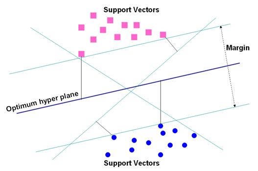
Figure 1: Optimum hyper plane for linearly separable data with support vectors.

Figure 2: Optimum hyper plane for the binary linearly separable data.

The optimum hyper plane is determined by solving
min(0.5*||w||2 )                                                                                                                    (14)
subject to constraints,
yn (w. xn + b ) ≥ -1   and yn  ε {+1, -1}                                                                              (15)

SVM can function both as a binary classifier and as a multi-class classifier. Figure 3 shows non-linearly separable data, is the case in various classification problems as in the classification of remotely sensed images using pixel samples. In such cases, SVM can be extended to allow for non-linear decision surfaces (Cortes and Vapnik, 1995; Pal and Mather, 2003).

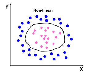Figure 3: Separation of non-linear data sets.

In such cases, the optimisation problem is replaced by introducing slack variable .

                                                                                                     (16)
subject to constraints
                                                                    (17)
where C is a regularisation constant providing equilibrium between margin maximisation and error minimisation, and  indicates distance of the wrongly classified points from the optimal hyper plane (Oommen et al., 2008). Larger the C value, higher is the penalty associated to misclassified pixels (Melgani and Bruzzone, 2004).

When the data cannot be represented linearly, non-linear mapping functions (Ф) are used to map them to a higher dimensional space (H). An input data point x is represented as Ф(x) in the high-dimensional space. The expensive computation of (Ф(x).Ф(xn)) is reduced by using a kernel function (Mathur and Foody, 2008a). Thus, the classification decision function is

        (18)                                                                                      

where for each of N training cases there is a vector (xn) that is the spectral response with class membership (yn). αn (n = 1,….., N) are Lagrange multipliers and K(x, xn) is the kernel function. The magnitude of αn is decided by C (Mathur and Foody, 2008b). The kernel function spreads the data points so that a linear hyper plane can be fitted (Dixon and Candade, 2008). Kernel functions commonly used in SVMs are broadly linear, polynomial, radial basis function and sigmoid. The choice of kernel functions and their parameters greatly influence the performance of SV models as we shall observe in this study. In this work, SVM classifier was executed with two types of kernels: polynomial, and radial basis function (RBF):

Polynomial:                                                                       (19)
RBF:                                                                     (20)

where, γ is the gamma term for all kernel types except linear, d is the polynomial degree, and r is the bias term. The correct selection of γ, d, and r significantly increase the accuracy of SVM (Chang and Lin, 2001; Wu et al., 2004; Hsu et al., 2007).